Examples
Using PQL, you can build your predictive query for any prediction, use case, or business problem, with all the instruments and metrics for fine-tuning your predictions available through an intuitive SaaS interface.
Translating Business Problems into Predictive Queries
The purpose of ML is to make predictions about the future and predictive queries excel at solving problems that require predictive answers. Generally, business predictions can always be framed as forward-looking questions that follow the “What would the answer to this question be?” format. This framing is crucial for creating an effective predictive query.
Crucially, you will need to answer the following two questions:
- What is the target? Essentially, this is the question you are trying to answer. For example, if you want to predict the total amount of purchases each user makes over the next seven days, then the "sum of purchases over the next seven days" is your target.
- Who/What is the entity? Namely, the entity is who you are making predictions for. For example, if you want to predict the total amount of purchases per user, then the user is your entity.
Some common business predictive queries include:
- How many customers are likely to churn in the next month?
- What will a business subsidiary’s revenue be this year?
- What would a customer be likely to purchase next?
Primary Commands
A predictive query's PQL statement requires at least two components:
- A
PREDICTclause that defines the target you want to predict (e.g., future sales), and; - A
FOR EACHclause that specifies the entity of your prediction (e.g., customers, stores).
PQL statements start with a PREDICT clause that defines your prediction value for an entity from a dimension table.
Possible targets for use in the PREDICT clause include:
- A static attribute of an entity that happens to be missing in the graph for some entities (e.g., dietary
preference of a customer) - An aggregation over future facts tied to an entity (e.g., sum of purchase values)
- Future interactions between this entity and other entities (e.g., items a user might buy)
- Relational operators applied to the above (e.g., whether sum of sales is greater than
zero)
After specifying the prediction target, you must include the FOR EACH clause to specify the entity you want to make predictions for. Only a primary key column of a dimension table can be selected for this field.
Additionally, PQL includes a WHERE operation to drop rows that do not meet the specified conditions. This can be used to drop entities that are irrelevant to your prediction or targets to exclude from your aggregation (i.e., when you are only interested in a subset of the table).
Other primary commands include ASSUMING for investigating hypothetical scenarios and evaluating the impact of your actions or decisions, and CLASSIFY/RANK TOP K for retrieving only the top ranked values for a prediction.
Kumo’s Predictive Query Reference contains a full list of commands, operators, and model planner options for use in your predictive queries.
Predictive Task Examples
| Task Name | Type |
|---|---|
| Age Prediction | Regression |
| Prediction of Movie Ratings | Regression |
| Lifetime Value | Temporal Regression |
| Active Purchasing Customer LTV | Temporal Regression |
| Active Purchasing Customer Churn | Temporal Binary Classification |
| Fraud Detection | Temporal Binary Classification |
| Next Item Category Prediction | Temporal Multiclass Classification |
| Probability of Liking an Item | Non-Temporal Classification |
| Item to Item Similarity | Static Link Prediction |
| Top 25 Most Likely Purchases | Temporal Link Prediction |
| Item Recommendation | Temporal Link Prediction |
| Top 25 "High Value" Purchases | Temporal Classification/Ranking |
Age Prediction (Regression)
The following predictive query predicts the age of all customers, for which you don't know the age.
PQL Approach:
PREDICT customers.age
FOR EACH customers.customer_id
Data:
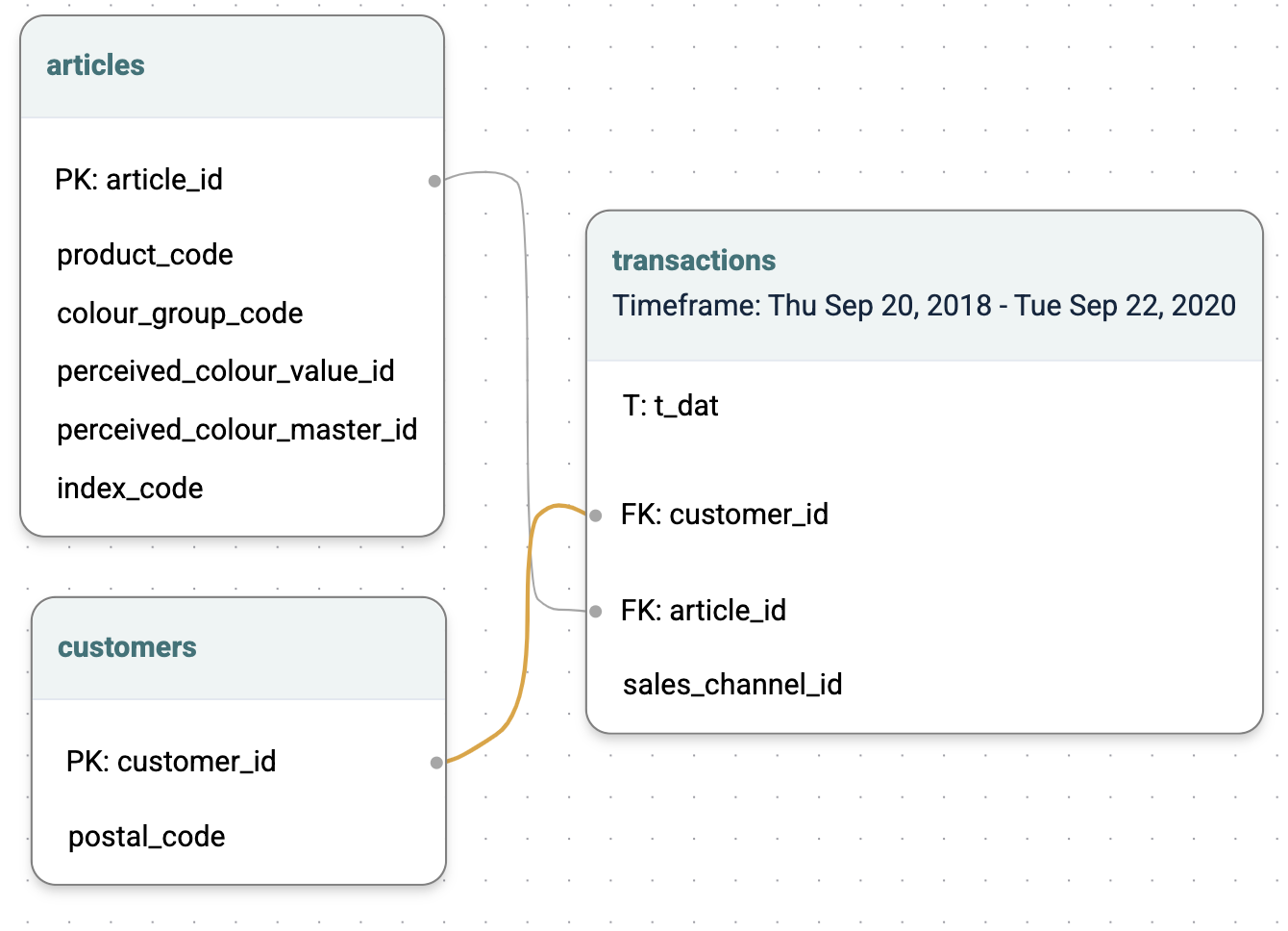
This predictive query is running on the following data schema:
customers: containing one row for each of your customers.transactions: containing one row for each transaction (purchase) made by each customer.articles: information about the products that the customer purchased.
Explanation:
This query is interpreted by Kumo as a regression task. It is regression because the prediction target age is a number. When the query is executed and a RandomSplit is used Kumo will randomly group the customers into train/val/test splits according to an 80/10/10 ratio. Model training will happen on the train and val splits, while evaluation will happen on the test split.
Prediction Output:
The batch prediction output is a table with two columns: customer_id and predicted age. Predictions will be made for all customers in the customers table, where age is null. In simple terms, you are predicting the age for all customers where their age is missing.
Prediction of Movie Ratings (Regression)
In this predictive modeling task, the objective is to forecast the rating a user might assign to movies that they have not yet rated. Your aim is to determine a continuous variable—movie ratings—by leveraging predictive variables from both user and movie domains.
PQL Approach:
PREDICT rating.rating
FOR EACH rating.ratingId
Data:
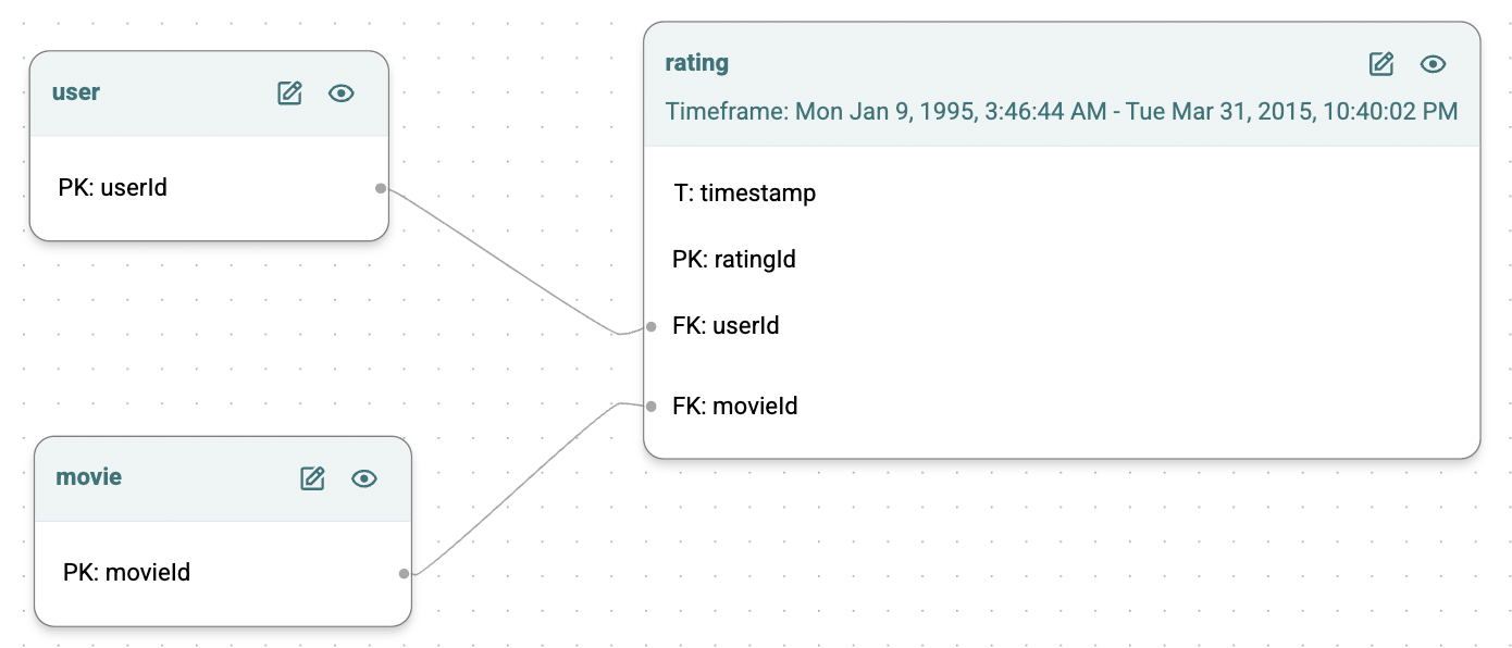
The ideal training dataset for this task would encompass three tables:
user: profile details like userId, age, gender, and other relevant features.movie: information such as movieId, genre, director, release year, and additional attributes.rating: contains ratingId, userId, movieId, and rating (1-5). Ratings are explicit if present; if null, they represent prediction opportunities for the model.
Explanation:
In PQL, the PREDICT function refers to the column to be predicted. The FOR EACH clause indicates your intention to create predictions for each individual rating entry (combination of user and movie) in the data set.
You employ the subset of data where users have rated movies to train your model, enabling it to discern the intricate relationships between users’ characteristics, their past rating patterns, the attributes of the movies, and the given ratings.
Prediction Output:
The end result is a structured table, where each row represents a distinct pairing of a user and a movie, together with a ratingId, complemented by a rating. This rating is the model’s prediction of how likely a user is to appreciate a movie, informed by the historical data and the inferred preferences from users with similar tastes and movie profiles.
Lifetime Value (Temporal Regression)
The following predictive query predicts how much each of your customers will spend over the next 30 days, a common measure of lifetime value (LTV). In this case, the entity is CUSTOMERS and the target is the SUM of TRANSACTIONS over the next 30 days.
PQL Approach:
PREDICT SUM(transactions.price, 0, 30)
FOR EACH customers.customer_id
Data:
This predictive query is running on the following data schema:
customers: containing one row for each of your customers.transactions: containing one row for each transaction (purchase) made by each customer.articles: information about the products that the customer purchased.
Explanation:
Because this query is predicting an aggregation SUM(), Kumo interprets this as a temporal predictive query. This means that Kumo will generate a set of train/val/test splits that cover the time range of the target table transactions. In this case, the target table has a time range of Sep 20, 2018 to Sep 22, 2020. Training examples will be generated by computing the 30-day spend of users, at various points in time during this time range.
This table will be used as labels for training a GNN model. Because the target of this query SUM() is a real-valued number, the task type of this query is regression, and the platform will export the standard evaluation metrics for regression, as described here.
Prediction Output:
The batch prediction output is a table with two columns: customer_id, and predicted SUM(transactions.price, 0, 30). Predictions will be made for all customers in the customers table, assuming an anchor time of September 22, 2020 (unless otherwise specified). This means that the model will predict the total spend of each customer, from September 22, 2022 until October 20, 2022.
Active Purchasing Customer Lifetime Value (Temporal Regression)
The following predictive query makes the same prediction as before, but only for actively purchasing customers (i.e., customers who made at least one purchase in the last 30 days).
PQuery Approach:
PREDICT SUM(transactions.price, 0, 30)
FOR EACH customers.customer_id
WHERE COUNT(transactions.*, -30, 0) > 0
Data:
This predictive query is running on the following data schema:
customers: containing one row for each of your customers.transactions: containing one row for each transaction (purchase) made by each customer.articles: information about the products that the customer purchased.
Explanation:
Training table generation is almost exactly the same as the previous example. However, in this case, training examples are only generated for users that had made purchases in the prior 30 days.
Prediction Output:
The prediction output format is the same as the previous example. However, predictions are only made for users that made purchases in the 30 days prior to the anchor time of September 22, 2020.
Active Purchasing Customer Churn (Temporal Binary Classification)
The following predictive query will predict whether an actively purchasing customer—defined as one that has made a purchase in the last 60 days—will go inactive by the end of the next 90 days.
PQL Approach:
PREDICT COUNT(transactions.*, 0, 90, days) = 0
FOR EACH customers.customer_id
WHERE COUNT(transactions.*, -60, 0, days) > 0
Data:
This predictive query is running on the following data schema:
customers: containing one row for each of your customers.transactions: containing one row for each transaction (purchase) made by each customer.articles: information about the products that the customer purchased.
Explanation:
Because PREDICT COUNT() = 0 is an true/false prediction per customer, Kumo treats this as a binary classification task. Because COUNT is an aggregation over time, this is treated as a temporal query, so it follow the same train table generation procedure that was described in the LTV example.
Prediction Output:
The batch prediction output is a table with two columns: customer_id, and a score containing the probability of COUNT(transactions.*, 0, 90, days) = 0. A prediction is made for every single customer that matches the WHERE condition at the anchor_time of batch prediction, which is September 22, 2020 by default.
Fraud Detection (Temporal Binary Classification)
In this predictive modeling task, your objective is to estimate whether a bank transfer was a fraudulent one. The final target is a boolean value—whether the transaction was (eventually) found to be fraudulent.
PQL Approach:
PREDICT fraud_reports.is_fraud
FOR EACH transaction.id
WHERE transaction.type = "bank transfer"
Data:
This task comes with the element of time: each transaction has a timestamp and when making the prediction, the model will only be able to access data with earlier timestamps. Moreover, you would assume that the fraud reports (i.e., the training labels) are inserted into the database with a time delay (because it takes time to obtain them). You would insert them as a separate table with their own corresponding timestamps. Each transaction with an available fraud report should contain the ID of its report, or N/A if a prediction needs to be made.
The ideal training dataset for this task would encompass three tables:
Users: profile details like User ID, age, gender, and other relevant features.Transaction: information such as transaction ID, Fraud report ID, transaction type, transaction date, transaction, amount, ID of the sender and receiver, and additional attributes.Fraud Reports: fraud Report ID, report timestamp, the label, and other possible information.
Explanation:
Transaction table contains several transaction types, but you only care about bank transfers. Adding an entity filter WHERE transaction.type = “bank transfer” will drop any training samples where the value of column type in table transaction is not “bank transfer”.
Important: The transaction table should contain a foreign key pointing to the fraud report table, and not the opposite way around. This way, at most one label exists per entity is guaranteed (at most one fraud report is linked to each transaction).
The data will get split with a TemporalSplit according to the time column of each entity (i.e., transaction). When making a prediction, the predictive model will only access data with smaller or equal timestamps.
Prediction Output:
The end result is a structured table, where each row represents a transaction without a fraud report and its corresponding predicted fraud label, complemented by a probability of a true and a false label. These scores are the model’s prediction of how likely a transaction is to be fraudulent, informed by the historical transactions and their labels. Transactions that do not meet the condition transaction.type = “bank transfer” will not be included.
Next Item Category Prediction (Temporal Multiclass Classification)
In this predictive modeling task, your objective is to predict the type of the next purchase that a customer will make in the next seven days.
PQL Approach:
PREDICT FIRST(purchase.type, 0, 7)
FOR EACH user.user_id
Data:
Suppose that you are given a dataset from a clothing retailer with all the user information, their past purchases (one item per purchase), and item descriptions. Each purchase is labeled with a type: online, in-store, third-party-reseller, etc.
This task comes with the element of time: each purchase has a timestamp and when making a prediction, the model will only be able to access data with earlier timestamps. Training labels are also dependent on the time: As you change the point in the past that we’re focusing on, the notion of what the user’s next purchase is, changes. Kumo uses this to generate diverse training samples by going back in history.
The ideal training dataset for this task would encompass three tables:
Users: profile details like User ID, age, gender, and other relevant features.Purchase: information such as User ID, Item ID, purchase date, purchase value, purchase type, and additional attributes.Items: item ID, item description, item size, and other relevant features.
Explanation:
The target is an aggregation (FIRST) over the next seven days. When generating the training data, Kumo will first determine which past timestamps to generate the training data for. These are so-called “anchor times”. In this case, it will take a timestamp every seven days from the latest timestamp in the purchase history to the earliest. So, if the last purchase was made on 2019-12-31, the following anchor times will be generated: 2019-12-24, 2019-12-17, 2019-12-10, …
For each pair (user, anchor time) a label will be computed, that is, the first purchase type that this user made in the seven days following the anchor time.
Note: Since theFIRSTaggregation is undefined if a user made no purchases in the seven days following the anchor time, such examples are automatically dropped unless you use theIS NULLfilter. All future predictions are thus made under the assumption that a user will buy something. This is different from aCOUNTaggregation, where “no purchases” would simply be given value0.
By default, the generated data will be split with a ApproxDateOffsetSplit, which will put the final seven days of data (i.e., the last anchor time) into the test set, the second-to-last seven days into validation, and the rest into the training set. It is important to be mindful of this when defining the aggregation horizon. Using a very large prediction horizon might result in insufficient data for the split—at least 3 anchor times are required for a healthy train/val/test split.
On the other hand, using a very small aggregation window on a dataset with a long history might result in far too many generated examples, slowing down the training. To prevent this, use the train_start_offset parameter in the model plan. For example, train_start_offset: 300means that only the last 300 days are used for label generation.
During the training, model will only be able to access rows in the database with a timestamp smaller than the timestamp of the training sample in question, guaranteeing no data leakage.
Prediction Output:
When making predictions for the future, you need to specify the batch prediction anchor time—the point in time from which the prediction is made. By default, this will be the largest timestamp in the purchase table. The predictions are then made for one aggregation (seven days) from that point onward, one for each entity.
The end result is a structured table, where each row represents a prediction for a user with their corresponding predicted next purchase category, complemented by a probability of each class. These scores are the model’s prediction of how likely the user is to buy from that category next.
Probability of Liking an Item (Non-Temporal Classification)
The following predictive query will compute the probability that a user will "like" a particular item on your website. It defines a similar predictive task as a traditional Two Tower model used in recommender systems.
PQL Approach:
PREDICT customer_item_pairs.likes = 1
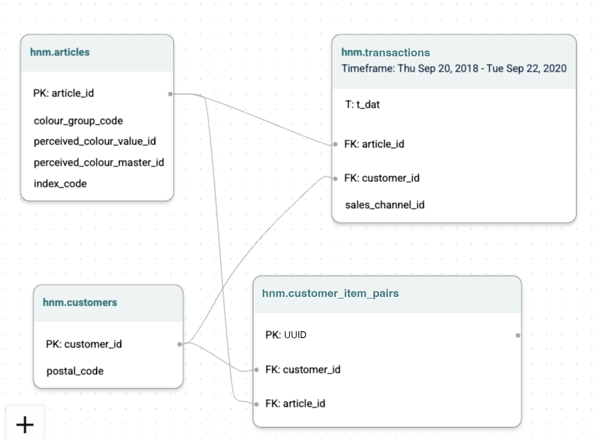
FOR EACH customers_item_pairs.uuidData:
This would require the same graph as above, but with the addition of a new table called customer_item_pairs which contains the "likes" signal. customer_item_pairs.likes would be a binary column with possible values of true, false, and null.
Explanation:
As the table of the predictive query customer_item_pairs does not contain a time column, this is a non-temporal query. Because this query is not temporal, Kumo will generate train/val/test splits by randomly distributing the rows of the customer_item_pairs table according to an 80/10/10 ratio. The label of the training table is defined by customer_item_pairs.likes = 1, and all rows where likes IS NULL are dropped.
Prediction Output:
The batch prediction output is a table with two columns: customer_item_pairs.uuid, and a score containing the probability that customer_item_pairs.likes = 1 . A prediction is made for every single uuid where customer_item_pairs.likes is null. In simpler terms, it makes a prediction for every single value that is missing.
Item to Item Similarity (Static Link Prediction)
In this predictive modeling task, your objective is to predict item similarity.
PQL Approach:
PREDICT LIST_DISTINCT(copurchase.dst_item_id) RANK TOP 10
FOR EACH src_item.item_id
Data:
Suppose that you are given a dataset with a set of items (including description, price, product details), and additional relational information (e.g., seller and buyer information). The ideal training dataset for this task would encompass three tables:
- A
source itemtable - A
destination itemtable - A
co-purchasetable between different items (e.g., pre-processed via Kumo views based on past purchase data)
Explanation:
The target is an aggregation (LIST_DISTINCT), without any window size, referring to a static link prediction task. The RANK TOP 10 clause dictates that we are interested in exactly 10 similar items per item. The generated data will by default be split with a RandomOffsetSplit, into 80% training, 10% validation and 10% test co-purchases.
For static link prediction tasks, two different module types are exposed:
- Ranking module: A link prediction GNN optimized for link prediction performance that produces the ranking scores directly. It can also produce embeddings, but their inner products are not perfectly aligned to the ranking.
- Embedding module: A model that optimizes link prediction with entity embedding outputs. The ranking scores can be obtained by fast vector calculations (default to inner product) on the embedding space.
Depending on the use-case and the downstream consumption of model outputs, a certain module type may be preferred over the other.
Another important configuration is whether the model needs to be able to handle new items at batch prediction time (inductive link prediction) or not (transductive link prediction), configured via the handle_new_target_entities model planner option. By default, Kumo assumes a transductive link prediction setting for best model performance. Inductive link prediction usually results in a bit lower model performance (since you cannot train corresponding lookup embeddings), but may be inevitable depending on the use-case.
In order to emphasize the learning of cold start items, you may additionally consider discarding the co-purchase table from being used inside the model. This can be achieved via the max_target_neighbors_per_entity: 0 option.
Prediction Output:
The end result is a structured table, where each row represents a missing co-purchase item pair, complemented by a score of this (user, user) pair. These scores are the model’s prediction of how likely the two items are co-purchased together. Given 10 recommendations per items, the final output will contain 10 times #src_items many rows.
Top 25 Most Likely Purchases (Temporal Link Prediction)
The following predictive query predicts the top 25 articles a customer is most likely to buy in the next 30 days. This is the best way to generate great product recommendations for users.
PQL Approach:
PREDICT LIST_DISTINCT(transactions.article_id, 0, 30, days)
RANK TOP 25
FOR EACH customers.customer_id
Data:
This predictive query is running on the following data schema:
customers: containing one row for each of your customers.transactions: containing one row for each transaction (purchase) made by each customer.articles: information about the products that the customer purchased.
Explanation:
Because LIST_DISTINCT and RANK result in a discrete list of articles, Kumo infers that this is a link prediction task. Intuitively, you are predicting which article_ids are most likely to have transactions for each user, in the next 30 days.
As LIST_DISTINCT is an aggregation over time, this predictive query is a temporal task, and follows the same training process as described in the LTV example.
Prediction Output:
The batch prediction output is a table with two columns: customer_id and PREDICTED, which contains the 25 articles that each customer is most likely to purchase in the next 30 days.
Item Recommendation (Temporal Link Prediction)
In this predictive modeling task, your objective is to predict the items that a customer will likely purchase next.
PQL Approach:
PREDICT LIST_DISTINCT(transactions.article_id, 0, 7) RANK TOP 10
FOR EACH customers.customer_id
Data:
This predictive query is running on the following data schema:
customers: containing one row for each of your customers.transactions: containing one row for each transaction (purchase) made by each customer.articles: information about the products that the customer purchased.
Suppose that this dataset is from a clothing retailer with all the user information, their past purchases (one item per purchase), and item descriptions. Users and items may come with additional time constraints (e.g., a timestamp of the user joining the platform, a timestamp for when this article became available, or when this article became sold out).
In particular, timestamps of articles play a crucial role in the predictive performance of your underlying machine learning model. Since “Item Recommendation” is mapped to a link prediction task, Kumo uses a contrastive loss formulation for training (i.e., past historical items are treated as positives, while non-existing purchases are treated as negatives). In order to ensure that negatives are correctly created, timestamps of items should be used whenever they are available, such that Kumo does wrongly use items that do not yet exist or do no longer exist as negatives.
Explanation:
The target is an aggregation (LIST_DISTINCT) over the next seven days. When generating the training data, Kumo will first determine which past timestamps to generate the training data for. These are so-called “anchor times”. In this case, it will take a timestamp every seven days from the latest timestamp in the purchase history to the earliest. So, if the last purchase was made on 2019-12-31, the following anchor times will be generated: 2019-12-24, 2019-12-17, 2019-12-10, … For each pair (user, anchor time) a list of item purchases will be computed. The RANK TOP 10 clause dictates that we are interested in exactly 10 item recommendations per user.
The generated data will by default be split with a DateOffsetSplit(), which will put the final seven days of data (i.e. the last anchor time) into the test set, the second-to-last 7 days into validation, and the rest into the training set.
It is important to be mindful of the window size in link prediction tasks. In particular, a small aggregation window may result in too few positives.
For temporal link prediction tasks, two different module types are exposed:
- Ranking module: A link prediction GNN optimized for link prediction performance that produces the ranking scores directly. It can also produce embeddings, but their inner products are not perfectly aligned to the ranking.
- Ranking module: A model that optimizes link prediction with entity embedding outputs. The ranking scores can be obtained by fast vector calculations (default to inner product) on the embedding space.
Depending on the use-case and the downstream consumption of model outputs, a certain module type may be preferred over the other.
Another important configuration is whether the model needs to be able to handle new items at batch prediction time (inductive link prediction) or not (transductive link prediction), configured via the handle_new_target_entities model planner option. By default, Kumo assumes a transductive link prediction setting for best model performance. Inductive link prediction usually results in a bit lower model performance (since we cannot train corresponding lookup embeddings), but may be inevitable depending on the use-case.
Prediction Output:
When making predictions for the future, you need to specify the “batch prediction anchor time”—the point in time from which the prediction is made. By default, this will be the largest timestamp in the purchase table. The predictions are then made for one aggregation (7 days) from that point onward, one for each entity.
The end result is a structured table, where each row represents a recommended item for a user, complemented by a score of this (user, item) pair. These scores are the model’s prediction of how likely the user is to purchase the item in the next seven days. Given 10 recommendations per user, the final output will contain 10 times #users many rows.
Top 25 "High Value" Purchases (Temporal Classification/Ranking)
The following predictive query predicts the 25 "high value" items a customer is most likely to buy in the next 30 days. "High value" items are defined to have price greater than $100.
PQL Approach:
PREDICT LIST_DISTINCT(
	transactions.article_id
  WHERE transactions.price > 100,
0, 30, days)
RANK TOP 25
FOR EACH customers.customer_id
Data:
This predictive query is running on the following data schema:
customers: containing one row for each of your customers.transactions: containing one row for each transaction (purchase) made by each customer.articles: information about the products that the customer purchased.
Suppose that this dataset is from a clothing retailer with all the user information, their past purchases (one item per purchase), and item descriptions. Users and items may come with additional time constraints (e.g., a timestamp of the user joining the platform, a timestamp for when this article became available, or when this article became sold out).
Explanation:
Almost everything is the same as the previous example, except for the addition of the WHERE clause within LIST_DISTINCT. This means that the training examples will only be created for transactions with price > 100.
Prediction Output:
The batch prediction output is a table with two columns: customer_id and PREDICTED, which contains the 25 articles, with price > 100, that each customer is most likely to purchase in the next 30 days.
Ranking tasks have a limit of 10 million target items—for more information, please see to the CLASSIFY/RANK TOP K pquery command reference.
Updated 2 months ago